Three insights from order quantity theory

In our last note, we discussed safety stock analysis — how to decide when to reorder. Here, we turn to the question of how much to order each time, using the classical Economic Order Quantity (EOQ) model.

Three key takeaways:

• The optimal order size balances capital costs (which favor small, frequent orders) against ordering costs (which favor larger, less frequent orders).
• The cost curve is forgiving — order frequency can deviate by up to a factor of $4$ from the optimum, and total cost will always stay within about $2\times$ the minimum. This gives flexibility in scheduling.
• This flexibility extends to seasonal demand: If fluctuations aren't extreme, you can stick to a fixed order cadence year-round without much penalty.

Examples and derivations follow — all geared toward intuition.

Review of the basic equations

According to the classical theory, optimal order volumes need to balance two competing costs:

• The holding cost of inventory: This is often set by interest that must be paid on loans used to purchase inventory – hold more inventory and you have to pay more interest, so this favors placing frequent, smaller orders.

• The cost of placing orders: E.g., it may cost some employee wage time to place each order, so this favors placing fewer, larger orders.

With just a little work, we can formalize these concerns and identify the optimal order volume. To begin, we first introduce the following variables:

• $D$ = annual unit demand
• $C$ = the annual cost of capital per unit – i.e., the unit cost times the interest rate
• $S$ = the cost to place a single order
• $Q$ = the amount we order each time

Now if $Q$ is ordered each time, and we reorder when inventory is close to zero, the average inventory level throughout the year will be about $Q/2$. The total cost of capital will then be

$$\begin{array}{c}\text{annual capital cost}=\frac{Q}{2}\cdot C\end{array}$$

The total number of orders that we must make throughout the year is $D/Q$. Each order costs $S$, so the total annual expense from placing orders is then

$$\begin{array}{c}\text{annual order placement cost}=\frac{D}{Q}\cdot S\end{array}$$

Combining these, the total cost is

$$\begin{array}{c}\text{total annual cost}=\frac{Q}{2}\cdot C+\frac{D}{Q}\cdot S\end{array}$$

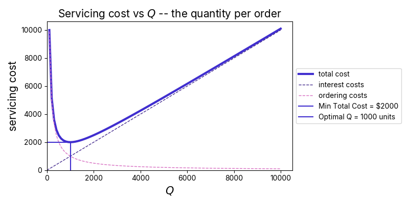
A plot of this function vs $Q$ is given below.

With some algebra, we find that the $Q$ value that minimizes (3) is

$$\begin{array}{c}\text{optimal order quantity}\equiv Q^{\ast }=\sqrt{\frac{2DS}{C}}\end{array}$$

This is the classical “Economic Order Quantity”. Notice that if either $D$ or $S$ goes up, we want to order more with each purchase, while if $C$ goes up we want to order less – makes sense! Plugging (4) into (3), we get

$$\begin{array}{c}\text{min total annual cost}=\sqrt{2DSC}\end{array}$$

Total costs go up if any of our three variables increase. Interestingly, at the optimal $Q$ the annual interest and ordering costs are equal in value – you can see this in the plot below, where the two dashed lines intersect at $Q^{\ast }$. Finally, dividing $D$ by $Q^{\ast }$, we get the optimal order frequency,

$$\begin{array}{c}\text{optimal orders per year}=\sqrt{\frac{DC}{2S}}\end{array}$$

This goes up with both annual demand and capital costs, but goes down with order placement cost.

Equations (4-6) are the standard results on order sizing theory. Below, we'll dig a little deeper to understand the cost of moving away from the optimal choice.

Figure 1: Plot of the costs incurred as a function of quantity ordered per purchase, $Q$. Here, we’ve set input parameters as follows: $D=10000$, $S=$ $$100$, and $C=$$$2$ (assuming $5\%$ annual interest rate, with an average unit cost of $$40$). In this case, the total cost is minimized with $Q^{\ast }=1000$, so that ten orders are placed each year. The total servicing cost is then $$2000$ for the year, with half coming from interest payments and half from the cost of placing orders.

Wiggle room about the minimum

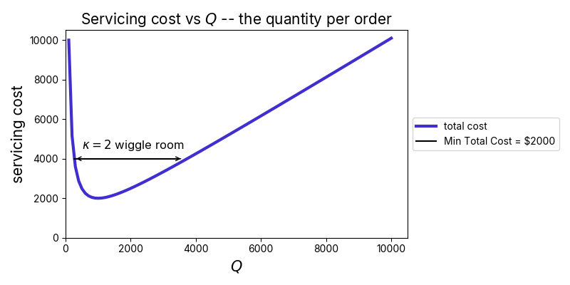
One nice thing about the total cost function near the optimal value is that it’s relatively insensitive to the exact order frequency / $Q$ value we opt to run with. That’s because the total cost function is flat there – it’s “derivative with respect to $Q$ is zero”. This means that we can adjust our order volume a bit and the total costs won’t go up that much. E.g., if instead of ordering $1000$ units each time, we instead opt to order $10000/12=830$ each time – so that we can order monthly for simplicity – the cost goes to $$2033$, a modest lift over the $$2000$ minimum.

To get precise, let’s now calculate the ‘wiggle’ room we have in setting $Q$. To do that, we’ll ask what values of $Q$ keep the costs within a range of $\kappa$ times the optimal choice. To find this, we set the total cost in (3) equal to this value, giving

$$\begin{array}{c}\kappa \sqrt{2DSC}=\frac{Q}{2}\cdot C+\frac{D}{Q}\cdot S\end{array}$$

This is a quadratic equation that we can solve for Q. The solution is

$$\begin{array}{c}Q=Q^{\ast }\times \left[\kappa \pm \sqrt{{\kappa }^2-1}\right]\end{array}$$

For example, if we set $\kappa \to 1$, we recover the unique optimal solution, $Q=Q^{\ast }$, as given in (4). However, if we set $\kappa \to 2$, we get

$$\begin{array}{c}Q=Q^{\ast }\times [2\pm \sqrt{3}]\sim Q^{\ast }\times [0.26,3.7].\end{array}$$

That is, we can order at a quantity that differs by almost a factor of $\sim 4$ either way from the optimal solution [1], and the net cost will only double – a universal result, independent of the specific parameters plugged in. Similarly, to keep costs within a factor of $\kappa =1.5$ of the minimum, our order quantity should be within a factor of $2.6$ or so of the optimal choice – relatively easy to hit.

We can leverage this flexibility to simplify our logistics. E.g., if a business carries multiple products, it may not be important to order each at its own specific optimal cadence. Instead, the business might group products into sets having relatively similar optimal order frequencies, and then order these all together at the same time. One set might be on a monthly cadence, another on a weekly, etc. So long as each product gets assigned to a group with order frequency that is not off by a factor of $4$ or more from its optimal cadence, costs will be within a factor of $\sim 2$ of the minimum possible.

Figure 2: As long as we place orders at a $Q$ that is not off from the optimal $Q^{\ast }$ by a factor of $4$ or more, the resulting cost will be no more than $\sim 2$ times the optimal value. This flexibility allows us to simplify ordering logistics without much cost – e.g., we can order all products at a common monthly cadence whose optimal order rate is not too far from that choice.

Seasonally-variable demand

Most businesses see demand fluctuate throughout the year in a seasonal manner, but the standard model we’ve discussed above neglects that. How can we adapt our solution above to this more realistic situation?

The approach we suggest is to reimagine the annual demand $D$ above to actually correspond to an annualized form of the monthly demand. For example, if net demand in the month of January is $d_{Jan}$, we’d write

$$\begin{array}{c}{D}_{Jan}=12\times d_{Jan}\end{array}$$

for the annualized version of January's demand, and so on for the other months. The optimal amount per order as set by this month's demand will then be given by

$$\begin{array}{c}{Q}_{Jan}^{\ast }=\sqrt{\frac{2D_{Jan}S}{C}}\end{array}$$

And the corresponding order frequency will be given by

$$\begin{array}{c}\frac{D_{Jan}}{Q_{Jan}^{\ast }}=\sqrt{\frac{C{D}_{Jan}}{2S}}\end{array}$$

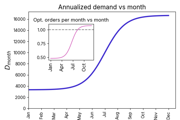
Is it important to seasonally adjust the order frequency to its optimal value, (12) – or at least some moving average version of this? Well from our analysis in the last section – not necessarily. It depends on how strong the seasonal profile is. If demand stays within a factor of $\sim 16$ of the average throughout the year – so that the optimal order frequency does not vary by more than a factor of $4$ – we can stick to any value within the range and never pay more than $2\times$ the optimal cost. Figure 3 below gives an example. However, in a case where the seasonal profile is quite strong, it may make sense to introduce two or more different ordering rates throughout the year. In this case, during busy seasons, the order frequency should go up, and in the slow seasons, it can relax – set as in (12).

Figure 3: Demand is plotted by month for a seasonal product. In the inset, we plot the optimal orders per month over the year as well – now also seasonal. However, because the optimal order frequency does not vary by more than a factor of $4$ over the course of the year, we can choose any convenient order rate within the span without incurring much cost. E.g., if we opt to order monthly – the gray dashed line in inset – costs will actually not be more than $50\%$ higher than optimal, even in the slow period.

Summary

In this post, we have extended our prior discussion on inventory management by introducing the Economic Order Quantity (EOQ) – the optimal amount of product to order that minimizes total annual costs. This balances ordering costs (e.g., administrative overhead) with holding costs (e.g., capital tied up in inventory). We have derived the classical EOQ formula and showed that this splits costs evenly at the optimum.

Importantly, the total cost function is flat near the optimum solution, giving businesses flexibility to adjust $Q$ for logistical convenience with minimal cost impact — within a factor of $2$ even if $Q$ is off by $\sim 4\times$. This last point can be applied to seasonal considerations, allowing businesses to stick to a fixed order frequency – unless seasonal fluctuations in demand are quite strong.

We plan one more review article on classical inventory management theory next time – stay tuned.

---

Thanks to Jaireh Tecarro for creating the banner image for this post.

[1] Interestingly, the wiggle room factors $[\kappa \pm \sqrt{{\kappa }^2-1}]$ are exact reciprocals of each other:

$$\begin{array}{c}\kappa +\sqrt{{\kappa }^2-1}=\frac{1}{\kappa -\sqrt{{\kappa }^2-1}}\end{array}$$

This is why we can talk of having to be within a given factor of the optimal order quantity or order frequency to hit a given cost lift factor – e.g., "You have to be within a factor of $\sim 4$ either way to avoid doubling the cost."